Membrane proteins (MPs) reside in the plasma membrane and perform various biological processes including ion transport, substrate transport, and signal transduction.*
Function-related conformational changes in membrane proteins occur in times scales ranging from nanoseconds to seconds.*
Obtaining time-resolved dynamic information of MPs in their membrane environment is still a major challenge.*
Although High Speed Atomic Force Microscopy (HS-AFM) images label-free samples such as DNA, soluble proteins, MPs, and intrinsically disordered proteins at ~1n~m lateral, ~0.1 nm vertical and ~100 ms temporal solution in aqueous environment and at ambient temperature and pressure, its temporal resolution is too slow to characterize many dynamic biological processes.*
In order to overcome this limitation Raghavendar Reddy Sanganna Gari, Joel José Montalvo-Acosta, George R. Heath, Yining Jiang, Xiaolong Gao, Crina M. Nimigean, Christophe Chipot and Simon Scheuring in their article Correlation of membrane protein conformational and functional dynamics use High Speed Atomic Force Microscopy Height Spectroscopy ( HS-AFM-HS) to characterize the microsecond timescale conformational changes of an integral-MP model system, i.e., the outer membrane protein G (OmpG) in a membrane environment.*
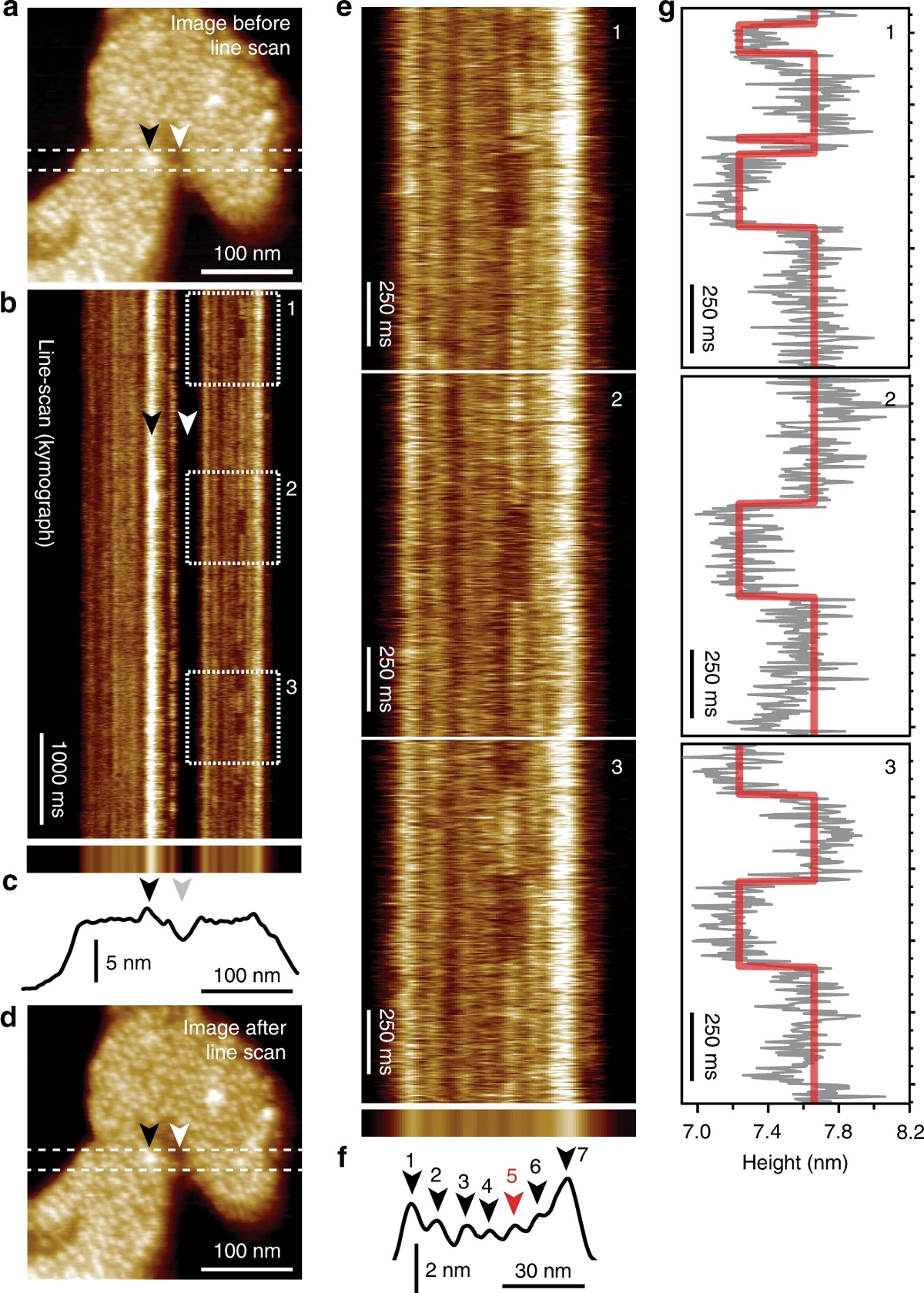
The positioning of the AFM tip is guided by HS-AFM imaging immediately before HS-AFM-HS-operation.*
NanoWorld Ultra-Short Cantilevers (USC) of the USC-F1.2-k0.15 type were used for the HS-AFM and HS-AFM-HS presented in the article.*
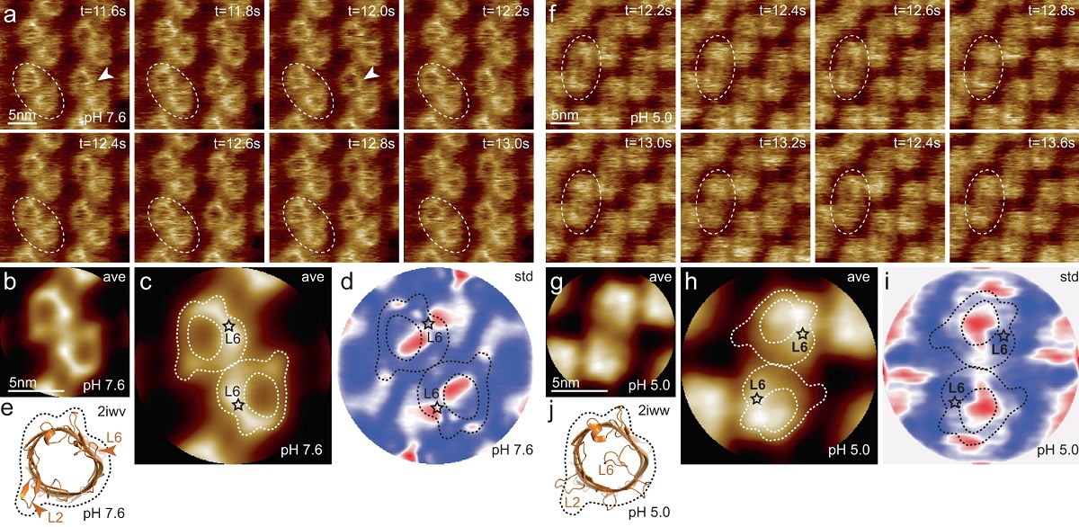
HS-AFM imaging of OmpG in lipid bilayers at pH 7.6 and pH 5.0.
a OmpG at pH 7.6 (Supplementary movie 1, left; frame rate: 200 ms per frame). A OmpG dimer is highlighted with dashed outline in all frames. Arrowheads in t = 11.6 s: Loop-6 fluctuating over the lumen. Arrowhead in t = 12.0 s: Fully open state. b Correlation average (n = 2752) of the HS-AFM movie frames (344 frames recorded over 68.8 s, full color scale: 0.0 nm < height < 1.25 nm, where the membrane level was set to 0.0 nm). c Correlation average of OmpG dimers. The topography outline (based on the molecular structure in 1e), serves as a visual guide to locate loop-6 and loop-2 in the topography and is highlighted by the dashed outline (the position of loop-6 is indicated by the asterisk based on its location in the structure (e)). Inner dashed outline show barrel lumen. d Standard deviation (std) map (n = 2752) from the averaging process in (b) (full color scale from blue to red: 0.05 nm < std < 0.19 nm) and topography outlines as in (c). e X-ray structure (PDB 2iwv) of the open OmpG conformation. Loop-6 (arrowhead L6) stands out of the image plane towards the viewer. Loop-2 (L2) forms a beta strand pointing away from the β-barrel, well detected by HS-AFM in the open state (b). f OmpG at pH 5.0 (Supplementary movie 1, right; frame rate: 200 ms per frame). A OmpG dimer is highlighted with dashed outline in all frames. g Correlation average (n = 2472) of the HS-AFM movie frames (309 frames recorded over 61.8 s, full color scale: 0.0 nm < height < 0.7 nm, where the membrane level was set to 0.0 nm). h Correlation average of OmpG dimers. For comparison, the topography outline of the open state (e) is shown (the position of loop-6 is indicated by the asterisk). i Standard deviation (std) map (n = 2472) from the averaging process in (g) (full color scale from blue to red: 0.04 nm < std < 0.07 nm) and topography outlines as in (h). j X-ray structure (PDB 2iww) of the closed OmpG conformation shown in the same orientation as in (e). Loop-6 (L6) folds over the β-barrel lumen in a lid-like manner. Loop-2 (L2) does not form a β-strand in the closed state, in agreement with absence of topography in this region in (h). Black dashed line: outline based on (e) for comparison.
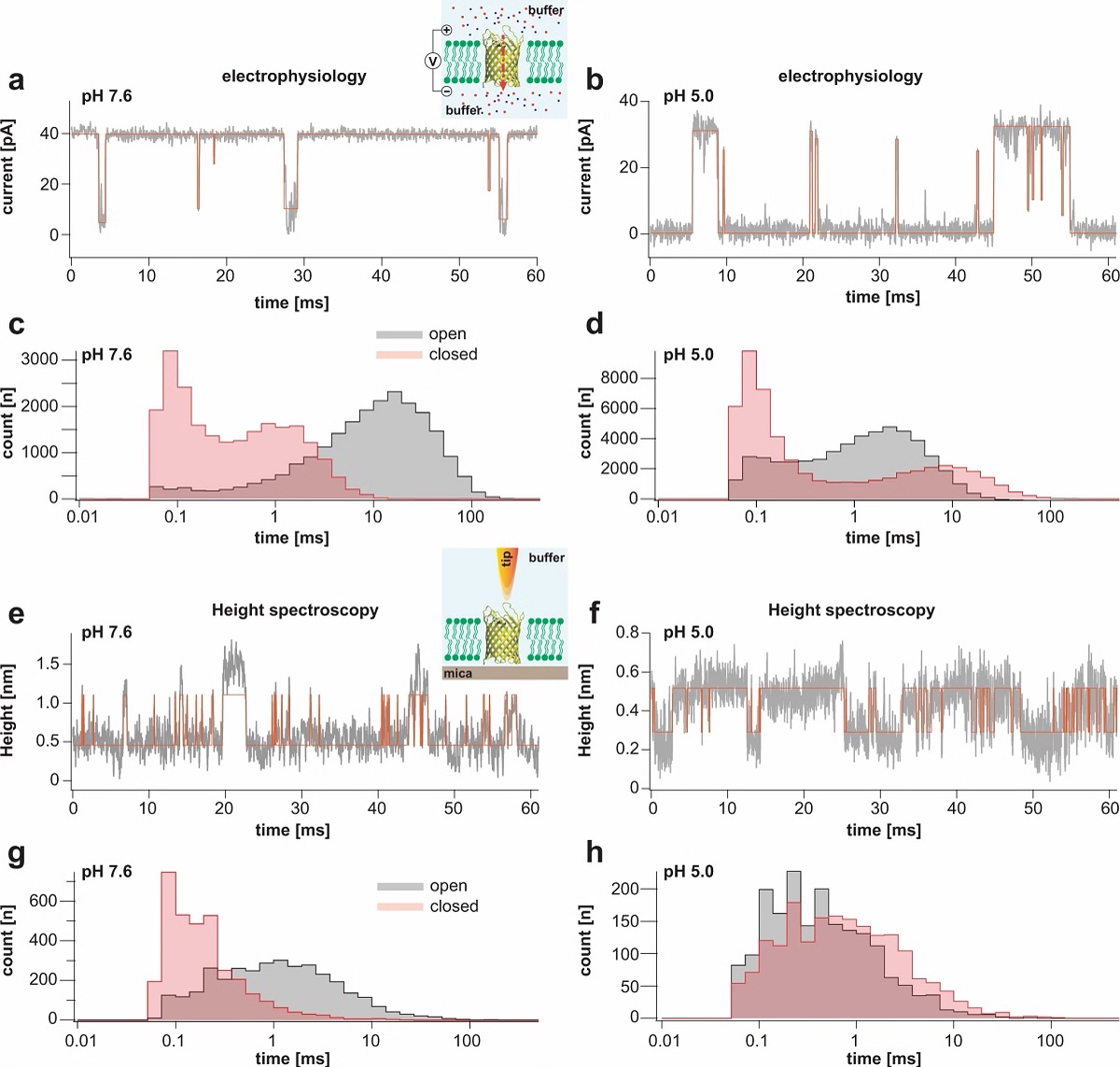
Single channel electrophysiology and HS-AFM height spectroscopy recordings of OmpG in lipid bilayers.
Representative 60-ms segments of OmpG single channel recordings at pH 7.6 (a) and pH 5.0 (b) at +40 mV membrane potential (longer traces in Supplementary Figs. 2 and 3). Cartoon representation of single channel recording experimental setup is shown in inset of (a). OmpG (yellow) in open state (PDB:2IWV) is placed in a lipid bilayer (green) surrounded by buffer (light blue shade) and potassium and chloride ions are shown as red and blue spheres. Red arrow indicates ion flow through OmpG in response to voltage application. Dwell time histograms of open and closed states at pH 7.6 (c) and pH 5.0 (d) from single-channel recordings (see Supplementary Table 1). Representative 60-ms segments of OmpG HS-AFM-HS recordings at pH 7.6 (e) and pH 5.0 (f) (longer traces in Supplementary Fig. 4). Cartoon representation of HS-AFM height spectroscopy experimental setup is shown in inset of (e). An oscillating AFM tip (orange) detects conformational changes of loop motion. Dwell time histograms of open and closed states at pH 7.6 (g) and pH 5.0 (h) from HS-AFM-HS recordings (Supplementary Table 2). In HS-AFM-HS the low state represents the open state, where the HS-AFM tip can descend into the β-barrel, and the high state represents the closed state, where loop-6 covers the beta barrel barring access of the HS-AFM tip to the cavity. All current-time and height-time traces were filtered at 20 kHz during analysis. The state dwell-time histograms are shown using log binning for better visualization of the components49. Red traces in (a) and (b) represent idealized current-time traces using clampfit software. Red traces in (e) and (f) represent idealized height-time traces using the STaSI algorithm (see Methods).
*Raghavendar Reddy Sanganna Gari, Joel José Montalvo-Acosta, George R. Heath, Yining Jiang, Xiaolong Gao, Crina M. Nimigean, Christophe Chipot and Simon Scheuring
Correlation of membrane protein conformational and functional dynamics
Nature Communications volume 12, Article number: 4363 (2021)
DOI: https://doi.org/10.1038/s41467-021-24660-1
Please follow this external link to read the full article: https://rdcu.be/cAE2S
Open Access : The article “Correlation of membrane protein conformational and functional dynamics” by Raghavendar Reddy Sanganna Gari, Joel José Montalvo-Acosta, George R. Heath, Yining Jiang, Xiaolong Gao, Crina M. Nimigean, Christophe Chipot and Simon Scheuring is licensed under a Creative Commons Attribution 4.0 International License, which permits use, sharing, adaptation, distribution and reproduction in any medium or format, as long as you give appropriate credit to the original author(s) and the source, provide a link to the Creative Commons license, and indicate if changes were made. The images or other third party material in this article are included in the article’s Creative Commons license, unless indicated otherwise in a credit line to the material. If material is not included in the article’s Creative Commons license and your intended use is not permitted by statutory regulation or exceeds the permitted use, you will need to obtain permission directly from the copyright holder. To view a copy of this license, visit https://creativecommons.org/licenses/by/4.0/.